|
Problem Set #1 -- word file
- Take a selfie with your laptop showing that you have successfully downloaded SPSS in the background of the photo. Attach the selfie to your homework.
- A recently conducted study showed that Connecticut drivers change lanes on the highway without using their signal 1.46 times per mile. What kind of statistic is cited in the previous sentence?
- That same study determined that Connecticut drivers are much more likely to change lanes without signaling when compared to the national average. Does that conclusion rest on an inferential or a descriptive statistic?
- I recently read a study designed to determine if exercise reduced depression in college students. A group of students was selected randomly from the campus directory. They rated their mood on a 10-point scale and indicated how many hours a week they went to the gym. The researchers found that, in general, people who spent more time in the gym reported being in better moods than people who spent less time in the gym. For the described study:
- Please identify the independent and dependent variables along with the operational definition for each.
- What type of scale of measurement are the IV and DV in?
- Was the study correlational or experimental?
- Can the researchers draw a cause-and-effect relationship between the variables of interest? If not, propose an alternative explanation for the reported results.
Problem Set #2 -- word file
- Make a frequency distribution table for the following data which includes the frequency and the relative frequency for scores:
| 74 | 103 | 95 | 98 | 81 | 117 | 105 | 99 | 63 | 86 | 94 | 107 |
| 96 | 100 | 98 | 118 | 107 | 82 | 84 | 71 | 91 | 107 | 84 | 77 |
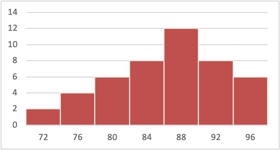
- Answer the questions below on the basis of this figure:
- Is this figure a bar graph or a histogram? Explain your answer.
- How many modes does the figure include?
- Is the figure positively-skewed, negatively-skewed or symmetrical?
- Calculate the sums of squares for the following set of data: 4, 6, 7, 8, 10.
- The numbers that follow represent the total number of hours of sleep that I received each night for the first week of the semester: 6, 7, 7, 6, 7, 4.5, 8. Find, the mean, median, and mode for these data. Show your work.
- Oddly, I wound up getting 12 hours of sleep one night during the third week of the semester. Which MCT would likely be most affected by that single anomalous datapoint?
Problem Set #3 -- word file
- The numbers that follow represent the total number of hours of sleep that I received each night for the first week of the semester: 6, 7, 7, 6, 7, 4.5, 8. Find, the variance and standard deviation for these data. Show your work.
- Let's say that the second week of the semester, the mean number of hours that I slept was exactly the same as it was for the first week, BUT, the variance was twice as large. For which week (first or second) would I be more likely to have gotten an unusually small (or large) amount of sleep? Explain your answer.
- Assume heights are normally distributed with a mean of 68 inches and a standard deviation of 4 inches.
- Use z-scores to determine the probability that an Amherst student is at least 5'3". Hint: consult the unit normal table, which can be downloaded from Moodle and/or the course website.
- Use z-scores to determine the proportion of people that are between 5'4" and 6'0" (i.e., at least 5.4", but not taller than 6'0"). Use the same procedure as in part a.
- If I select a person at random, what would we estimate is the probability they will be over 6'0"?
- A physical fitness association is including the mile run in its secondary school fitness test. The time for this event is approximately normally distributed with a mean of 450 seconds and a SD of 40 seconds. If the association wants to designate the fastest 10% as excellent what time should the association set as their cutoff?
Problem Set #4 -- word file
- Fill in the blanks: According to the central limit theorem, the ____________ distribution of a population will be approximately ____________ if n is sufficiently large (n > ________). Also, the population parameter should be equal to the mean of the ________________ and the ____________________ will be equal to σ/√n?
- What is the difference between:
- A sampling distribution
- A population distribution
- A sample distribution
- A researcher examines the relationship between delinquent behaviors and poor verbal abilities in teenagers. They administer a verbal IQ test to a sample of 81 incarcerated juvenile delinquents, you find that the sample mean verbal IQ is 103. The verbal IQ test is known to have a μ= 107 and aσ = 15 in the general population of teenagers.
- Assuming that the population mean and SD for juvenile delinquents is the same as that for the general population of teenagers, what is the probability of selecting a sample with a mean of 103 or lower?
- Do you think that juvenile delinquents have the same population mean and SD for verbal IQ as the general population of teenagers? Explain your answer.
Problem Set #5 -- word file
- In a previous problem set, I told you that these were the number of hours of sleep that I had received each night for the past week: 6, 7, 7, 6, 7, 4.5, 8. Last time I asked you to find the mean, median, mode, variance and standard deviation for these data.
- Now I want you to find the 90% and 95% CI for the average number of hours I sleep per night based on the numbers I obtained for that week.
- Provide an interpretation of what each CI tells us.
- It is known that if people are asked to make an estimate of something, for example, 'how tall is Johnson Chapel?'' the average guess of a group of people is more accurate than an individual's guess. Vul and Pashler (2008) wondered if the same held for multiple guesses by the same person. They asked people to make guesses about known facts. For example 'what percentage of the world's airports are in the United States?'' Three weeks later the researchers asked the same people the same questions and averaged each person's responses over the two sessions. They asked whether this average was more accurate than the first guess by itself.
- Using the principles of hypothesis testing we have learned (not necessarily the rules for one type of test), in English, what would be the null and alternative hypothesis?
- What conclusion would represent a Type I and a Type II error for this study?
Problem Set #6 -- word file
- Williamson (2008) conducted a study to examine psychological adjustment among children of parents with depression. Williamson expected that children with at least one parent with depression would show unusually high levels of behavior problems. To examine this, a sample of 166 children with at least one parent with depression was recruited. They were given the Youth Self-Report Inventory, which is a nationally normed measure with a population mean of 50 and a standard deviation of 10; higher scores on this measure indicate greater behavior problems. Williamson obtained a sample mean of 55.71. Conduct a one-sample hypothesis test to determine if children of parents with depression have greater behavior problems than typical children (Steps 1 to 8). Set α to .05.
Step 1: Decide whether you are conducting a one- or a two-tailed test.
Step 2: Specify the NULL hypothesis (HO).
Step 3: Specify the ALTERNATIVE hypothesis (HA).
Step 4: Designate the rejection region by selecting α.
Step 5: Determine the critical value of your test statistic.
Step 6: Use sample statistics to calculate test statistic.
Step 7: Compare observed value with critical value.
Step 8: Interpret your decision regarding the null.
- You get a job as a traveling salesperson for Callahan Brake pads. You try to sell your first client on the idea that Callahan Brake pads are superior in quality. The client is concerned about price. So, you conduct a study to convince him that Callahan brake pads do not cost any more or less than the average brake pad. Callahan Brake pads cost $15 per pair. The average cost of your 5 leading competitors $13.62 with s = 1.09. Conduct a one-sample hypothesis test (α = .05) to determine if the cost of Callahan Brake pads are in fact different from average (Steps 1 through 8). Be sure to interpret your results and to report the test statistics appropriately. Set α to .05.
Step 1: Decide whether you are conducting a one- or a two-tailed test.
Step 2: Specify the NULL hypothesis (HO).
Step 3: Specify the ALTERNATIVE hypothesis (HA).
Step 4: Designate the rejection region by selecting α.
Step 5: Determine the critical value of your test statistic.
Step 6: Use sample statistics to calculate test statistic.
Step 7: Compare observed value with critical value.
Step 8: Interpret your decision regarding the null.
- Research suggests that people are more likely to gamble if they are in a good mood. Professor Keno and Professor Roulette want to replicate this finding. They agree to manipulate mood by showing their subjects hilarious cat videos on youtube. They also agree to assess willingness to gamble using a standard measure in the field. However, Professor Keno uses two groups of subjects: one group watches a hilarious cat video before completing the gambling measure; the other does not. Professor Roulette has her subjects complete the gambling measure twice: once after watching a hilarious cat video and once after watching an emotionally neutral do-it-yourself video about home composting. Which professor – Keno or Roulette – constructed an experiment that should be analyzed as a paired sample t-test? Explain.
- You and Biff are playing a heated game of Jacks, when the conversation invariably turns to who is the superior player. You both know enough statistics to know that one game won't settle the matter completely. So, you each play six games, you pick up 5, 4, 8, 4, 5, and 6 jacks. Biff picks up 4, 4, 5, 3, 4, and 5 jacks.
- Conduct a hypothesis test (α = .05) to determine who is the better jackster (Steps 1 through 8). Be sure to interpret your results and to report the test statistic correctly. Set α to .05
Step 1: Decide whether you are conducting a one- or a two-tailed test.
Step 2: Specify the NULL hypothesis (HO)
Step 3: Specify the ALTERNATIVE hypothesis (HA)
Step 4: Designate the rejection region by selecting a.
Step 5: Determine the critical value of your test statistic
Step 6: Use sample statistics to calculate test statistic.
Step 7: Compare observed value with critical value
Step 8: Interpret your decision regarding the null including an approriate measure of effect size.
Problem Set #7 -- word file
- Two students are conducting a class project to determine whether music is a better cue for autobiographical memories than pictures or words. They kind of get their wires crossed so they don’t run the experiment the exact same way. Carrie gives each of her subjects three cues – a song, a picture, and a word (counterbalancing the order). Julia gives one group of students a musical cue, and a separate group of subjects a pictorial cue and a third group a word cue. Which design operationalized cued type (music vs. picture vs. word) as a within subject variable? Explain.
- Do people experience higher emotional well-being when exposed to sunshine? To test this, a researcher recruits a sample of 8 people. She asks them to complete a questionnaire measuring their emotional well-being when they are exposed to high levels of sunshine and then again when they’re exposed to low levels of sunshine. Conduct a t-test to determine if sunshine affects subjective feelings of well-being (Steps 1 through 8). Be sure to interpret the results and report the test statistic correctly. Set α at .05.
|
Person 1 |
Person 2 |
Person 3 |
Person 4 |
Person 5 |
Person 6 |
Person 7 |
Person 8 |
Low |
14 |
13 |
17 |
15 |
18 |
17 |
14 |
16 |
High |
18 |
12 |
20 |
19 |
22 |
19 |
19 |
16 |
Step 1: Decide whether you are conducting a one- or a two-tailed test.
Step 2: Specify the NULL hypothesis (HO)
Step 3: Specify the ALTERNATIVE hypothesis (HA)
Step 4: Designate the rejection region by selecting a.
Step 5: Determine the critical value of your test statistic
Step 6: Use sample statistics to calculate test statistic.
Step 7: Compare observed value with critical value
Step 8: Interpret your decision regarding the null including an appropriate measure of effect size.
Problem Set #8 -- word file
- Researchers conducted an experiment to examine if physical contact reduces perceived pain. Subjects are exposed to a repeated mild shock and are randomly assigned to one of three conditions. In one condition they are alone while the shock is administered (Alone condition). In a second condition a stranger is present in the room while the shock is administered (Physical presence condition). In a third condition, a stranger is present in the room and holds the participant’s hand while the shock is administered (Physical contact condition). Participants rate their subjective feeling of pain on a 1 to 10 scale with higher scores indicating more perceived pain. Conduct a one-way ANOVA to determine if condition influences perceived pain (set α to .05). Be sure to report the results of your F-test correctly and to conduct post-hoc tests if warranted; note that the critical value for q for this problem is 3.95. Based on the results of your test, what recommendation would we make to hospital staff working with patients undergoing painful procedures? Why?
Alone |
Physical Presence |
Physical Contact |
x |
x2 |
x |
x2 |
x |
x2 |
10 |
|
7 |
|
4 |
|
8 |
|
8 |
|
5 |
|
9 |
|
7 |
|
3 |
|
6 |
|
9 |
|
5 |
|
|
|
|
|
|
|
|
|
|
|
|
|
- A psychologist was interested in how children learn. She conducted an experiment in which 2 year-old children learned where an object was hidden by watching a video. The children either watched the video passively (we’ll call this the Watch group), or had the opportunity to advance the video by touching the screen anywhere (General Touch group) or in specific, ‘logical’ locations; that is a location that made sense given the way the video had played out up to that point (Specific touch). Learning was assessed by determining whether the children could find the object shown in the video in a real world version of the video scene; there were 15 trials. Twenty children participated in each group. The data were analyzed and the group means and ANOVA table appear below. Again, the dependent measure was the number of times the child found the hidden object, so higher scores indicate better learning. Interpret the results and make a conclusion about the ANOVA test; conduct post-hoc tests if appropriate (critical value for q = 3.40). Provide a final write-up of the results using proper statistical notation and report of the means. Set α to .05
General Touch Mean (n = 20) |
Watch Group (n = 20) |
Specific Touch Mean (n = 20) |
8.70 |
5.90 |
11.20 |
Source |
SS |
df |
MS |
F |
p |
| Between Treatment |
281.20 |
2 |
140.60 |
29.34 |
.001 |
| Within Treatment |
273.20 |
57 |
4.793 |
|
|
| Total |
554.40 |
59 |
|
|
|
Problem Set #9 -- word file
- Below are the results of a one-way ANOVA with three treatments. In each treatment there were 8 participants (n = 8).
- Fill in the missing values below (HINT: start by computing the degrees of freedom):
Source |
SS |
df |
MS |
F |
| Between Treatment |
40 |
|
|
|
| Within Treatment (error) |
|
|
4 |
|
| Total |
|
|
|
- The four sources of variability in a repeated measures ANOVA design are described below. Match each definition with the correct source: total variability; between treatments variability; within treatments variability; between subjects variability.
- The scores in the data set as a whole are relatively spread apart or relatively bunched together.
- The scores in treatment are relatively close to one another or relatively spread apart.
- The means are relatively similar to the Grand Mean or are relatively dissimilar from the Grand Mean.
- The scores of the participants are relatively similar to one another or are relatively different from one another.
- If the between participants variability is relatively high, will that increase or decrease the likelihood of rejecting the null hypothesis? Explain your answer.
- A researcher wants to examine a new social skills treatment to improve friendships in children. She recruits 6 children to participate in the treatment. The number of friends each child has is assessed before treatment begins, 3 months into treatment and 6 months into treatment. She wants to examine if time in treatment influences number of friendships. The data are presented in the table below. Conduct a repeated measures ANOVA by hand to determine if there is a significant effect of duration of treatment on unruly behavior (set α = .05). You do not have to run post-hoc tests.
|
Before |
3 month |
6 months |
P |
Billy |
0 |
4 |
2 |
|
Bobby |
1 |
5 |
6 |
|
Bubby |
3 |
3 |
3 |
|
Benny |
0 |
1 |
5 |
|
Barry |
0 |
2 |
4 |
|
Biff |
2 |
3 |
4 |
|
Mean |
|
|
|
|
T |
|
|
|
|
∑ (X2) |
|
|
|
|
Problem Set #10 -- word file
- 1. A small study was conducted to examine whether expertise and/or empathy affect helping behavior. A confederate in a computer lab pretended to have trouble getting a computer program to run. The subjects in the experiment were either Novices (Intro to Computer Science students) or Experts (senior Computer Science majors). The subjects were also classified as being low or high in empathy on the basis for a short survey. The dependent measure was how many minutes passed before the subject attempted to help the confederate. The data are presented in the table below.
- Conduct a Two-Way ANOVA by hand to determine if there is a significant relationship between the variables in question (set α = .05). For the omnibus test, Fcrit = 3.24; for the main effects and interaction effect test, Fcrit = 4.49. Be sure to report the F statistics appropriately and to describe and interpret any significant main effects or interactions.
- If an interaction exists, sketch a graph of the effect
|
Novice |
Expert |
Low |
Sum(x) = 15
Mean = 3
Sum(x2) = 47 |
Sum(x) = 20
Mean = 4
Sum(x2) = 86 |
High |
Sum(x) = 15
Mean = 3
Sum(x2) = 51 |
Sum(x) = 5
Mean = 1
Sum(x2) = 7 |
- Fill in the blanks of this ANOVA table .
| Source |
SS |
df |
MS |
F |
p-value |
| Model |
|
|
34.00 |
|
.001 |
| Error |
|
|
|
|
|
| Total |
2000.00 |
224 |
|
|
|
| Source |
SS |
df |
MS |
F |
p-value |
| A |
|
2 |
42.00 |
|
.006 |
| B |
|
2 |
|
|
.025 |
| AxB |
|
4 |
|
4.00 |
.004 |
Problem Set #11 -- word file
- A researcher conducts a study looking at the relationship between volunteer work and two variables: empathy and anxiety. The subjects were asked to indicate how much time they spent volunteering at various community organizations (e.g., Amherst Survival Center); this was the dependent measure. The subjects were also asked to complete quick measures of empathy and anxiety (predictor variables). Statistical analyses indicated that the correlation between volunteering and anxiety was -.80; the correlation between volunteering and empathy was .40.
- Were people more or less likely to volunteer if there were more anxious? Explain.
- Was the relationship between helping and volunteering stronger or weaker than the relationship between volunteering and anxiety? Explain.
- Starbucks is looking for a new marketing angle so they decide to target college students. They want to show that drinking coffee makes you work harder. They decide to collect some data to support their claim. They approach students at the end of the day and ask them to report the number of cups of coffee they drank (X) and the number of hours worked in the library (Y). The data is below.
- Calculate a pearson correlation and interpret the association.
X |
Y |
X2 |
Y2 |
X*Y |
1 |
7 |
|
|
|
4 |
2 |
|
|
|
1 |
3 |
|
|
|
1 |
6 |
|
|
|
2 |
0 |
|
|
|
0 |
6 |
|
|
|
2 |
3 |
|
|
|
1 |
5 |
|
|
|
∑x = |
∑y = |
∑x2 = |
∑y2 = |
∑xy = |
- Should Starbucks worry that caffeine consumption has detrimental effects on work ethic? Why or why not?
Problem Set #12 -- word file
- Answer the following question on the basis of the SPSS output below which was generated from a regression analysis examining the relationship between anxiety and mistakes made during an honors thesis defense (this was an example we looked at during the correlation chapter).
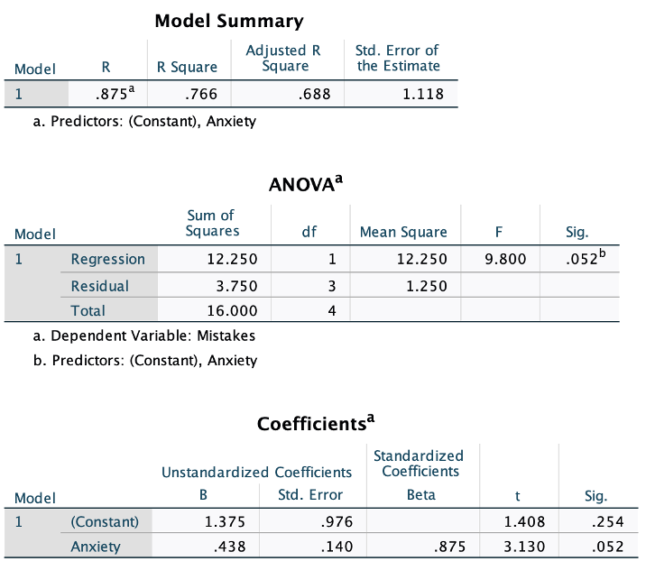
- What was the regression equation relating anxiety to mistakes?
- Was anxiety a significant predictor of mistakes?
- How much of the variance in mistakes could be attributed to variability in anxiety?
- You and Biff were sitting around one weekend evening, sipping on some age-appropriate refreshments (i.e. “Beer”). You noticed that as you drank more and more refreshments, your need to visit the bathroom (BR) increased. What are you going to do? You decide to collect some data. The table below presents information on a randomly selected sample of students for whom two pieces of data were collected: the number of refreshing beverages consumed in an evening, and the number of trips to the BR. Use these data to perform the following calculations:
X (beers) |
Y (trips to the BR) |
X2 |
Y2 |
X*Y |
3 |
0 |
|
|
|
4 |
2 |
|
|
|
5 |
5 |
|
|
|
5 |
5 |
|
|
|
4 |
6 |
|
|
|
7 |
8 |
|
|
|
4 |
2 |
|
|
|
6 |
4 |
|
|
|
5 |
3 |
|
|
|
7 |
5 |
|
|
|
|
|
|
|
|
|
|
|
|
|
- What is the linear regression relating beer consumption and trips to the BR?
- How many trips to the BR would you predict someone would make if they consumed 5 beers?
- Could you make a prediction for someone who drank a 12-pack? Explain.
- Is the y-intercept an interpretable value? If so, what does it suggest?
- Perform an ANOVA (not correlation) hypothesis test to determine whether the number of beers consumed is a significant predictor of trips to the BR.
- How much of the variance in trips to the BR can be explained by beer consumption?
- Here are the data in an SPSS file. Feel free to use this file and SPSS to check your answers.
Problem Set #14 -- word file
- Answer the following question on the basis of the SPSS output below which was generated from a multiple regression analysis examining the relationship between friendship quality and a variety of predictors. The subjects were asked to rate the quality of their friendship (e.g., how close they felt to the friend) along with several measures of similarity including: similarity of experiences, interests, and personality. The subjects also indicated how long they have been friends with the person (length) and whether they felt they could rely on their friend when they needed help (reliability).
| Source |
Sums of Squares |
df |
Mean Square |
F |
p-value |
| Model |
181.44 |
6 |
30.24 |
9.33 |
.001 |
| Error |
272.16 |
84 |
3.24 |
|
|
| Total |
453.60 |
90 |
|
|
|
| Variable |
df |
Parameter Est. |
Std. Err. |
t |
p-value |
| Intercept |
1 |
4.52 |
3.79 |
1.19 |
.236 |
| Experience |
1 |
6.42 |
2.13 |
3.01 |
.003 |
| Interests |
1 |
1.67 |
0.58 |
2.88 |
.005 |
| Personality |
1 |
-1.23 |
1.16 |
-1.06 |
.292 |
| Length |
1 |
1.98 |
0.56 |
3.54 |
.001 |
| Reliability |
1 |
-2.65 |
1.45 |
-1.83 |
.071 |
- What is the regression equation relating friendship quality to the predictor variables?
- What are the significant predictors of friendship quality?
- Would you be concerned if you found that there was a high correlation between Interests and Personality? Explain.
- How much of the variance in friendship quality could the model explain?
- Which factor(s) would you recommend removing from the model?
- Let's assume that the regression analysis was re-conducted after removing the factors that you identified in response to question e). r2 for the reduced model dropped to .378. Would you keep this original model or adopt the simpler reduced model even though it explained less of the variance in friendship quality? Explain.
|